Design a re-entrant auxetic structure, simulate it with FEM, and 3D print it in TPU.
blog.hirnschall.net


In order to analyze the natural frequencies of a given part, a 3D model with realistic material parameters can be used.
As the eigenfrequencies and eigenmodes are solutions to the generalized eigenvalue-problem $$A\eta = (2\pi f)^2 M\eta$$ we can approximate the solutions on a finite element space using the finite element method (FEM or FEA).
Although there are multiple different ways to solve this equation, we will use iterative methods to minimize the rayleigh-quotient. This makes sense as we are interested in the smallest eigenvalues and both \(A\) and \(M\) can be very large matrices (making an LU-factorization infeasible).
As an example, we will analyze the eigenfrequencies and eigenmodes of a tuning fork. If you are interested in more details you can watch our talk below or download the corresponding pdf.
As mentioned above, we will try to approximate solutions to the generalized eigenvalue problem $$A\eta = (2\pi f)^2 M\eta$$ within a finite element space.
We will therefore start by constructing a mesh for our geometry.

If we now use one hat function \(\phi_i\) per mesh vertex \(x_i\) such that $$ \phi_i(x_j)=\delta_{ij} $$ as basis for a space \(V_h\subset H^1_0\), we can represent each element of \(V_h\) as a linear combination of basis functions. This also applies to the approximation $$\eta^{(h)}=\sum_{j=1}^n \eta_j\phi_j$$ of \(\eta\) within \(V_h\).
Note: In practice, we will use the hat functions mentioned above in combination with higher-order basis functions to get a better approximation.


As our tuning fork is made out of metal, which deforms linearly (up to a point) we can use the model of linear elasticity to define the bilinear form \(a\) with Lamé parameters \(\mu\) and \(\lambda\) as $$ a:=\int_{\Omega} 2\mu\varepsilon(u):\varepsilon(v)+\lambda \operatorname{div}(u)\operatorname{div}(v)dH^n $$ where \(\varepsilon(u):= \frac{1}{2}\left(\nabla u +\nabla u^T\right)\) and \(C:D:=\sum_{ij}C_{ij}D_{ij}=tr(C:D^T)\). And the bilinear form \(m\) as $$ m:=\int_{\Omega}\rho uvdH^n. $$ As both \(a\) and \(m\) are bilinear we can define the stiffness-matrix \(A\) and mass-matrix \(M\) using the basis-functions \(\phi\) as $$ \displaylines{(A_{ij}):=a(\phi_i,\phi_j)\\ (M_{ij}):=m(\phi_i,\phi_j)}. $$ Note that both \(A\) and \(M\) are material dependent.
Now that we have constructed a mesh, a finite element space as well as the stiffness-matrix \(A\) and mass-matrix \(M\) we can use the LOPCG method (A. Knyazev 2000) to approximate the smallest eigenvalue and corresponding mode shape by minimizing the rayleigh-quotient. You can see the LOPCG algorithm below:
For this example, we have implemented the LOBPCG method (block version of LOPCG) using python/NGSolve. You can download the code in the download section below.
Here we have used Dirichlet boundary conditions on the handle of the tuning fork. You can see the resulting frequencies and mode shapes below:


Note: To make the talk more YouTube friendly we have simplified several aspects and we have omitted the somewhat technical proof for the rate of convergence of PINVIT (A. V. Knyazev and Neymeyr 2003).
We compare different iterative methods (including LOBPCG (A. Knyazev et al. 2007)) for computing eigenfrequencies and the corresponding eigenmodes in a finite
element space. We analyze both numerical complexity and convergence of each
algorithm and provide reference implementations using NGSolve.
The most suitable method is then used to analyze a clamped-free beam and a
tuning fork with realistic material properties.
We compare our results to the Euler-Bernoulli beam-theory and measurements
done on a real world model.
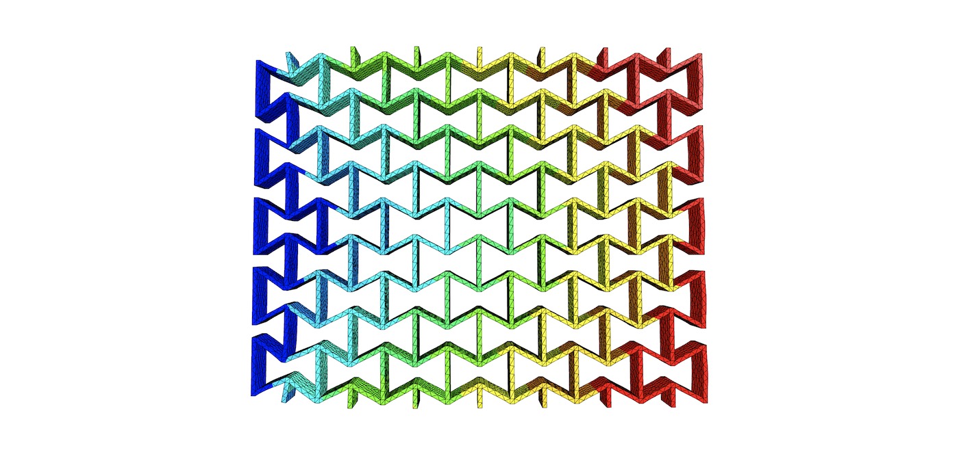
Design a re-entrant auxetic structure, simulate it with FEM, and 3D print it in TPU.
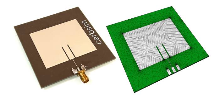
Convert Gerber files to a simulation-ready STEP file with full copper geometry (defeatured) — free tool for EM simulation.


