Eliminate manual bit packing errors with compile-time validation and code generation — full C++ implementation included.
blog.hirnschall.net


What if you could solve Formula Student rules quiz problems without thinking about them? While this may sound too good to be true, it has to work in theory and as it turns out, it also does in practice!
Each year the Formula Student rules quiz is a challenge. The questions can be daunting and if you do not want to end up on the FSG waiting list you better come prepared.
The questions themselves can be quite different from year to year. However, the core concept remains consistent. If you know the physics based equations/formulas required in the exercises you should be able to solve most of them.
This brings up an interesting idea. What if we build a very large system of equations using all physics based principles we know together with the information provided in the problem. If we then solve for any unknowns that are solvable we should get the solution to the problem.
To get this to work we need to do the following:
To do this efficiently and be able to easily create multiple tools for different fields, e.g. aerodynamics, vehicle dynamics, motor, etc. We will use multiple git repositories and integrate them into each other as a submodule. The main blocks will be
Let's tackle these challenges one by one.
To define the equations we will use a template system. Each equation template will define the actual equations, the variables used in the equations along with a description, which variables need to be known in order to have any chance or solving the equations, and the name of the equations (used for nice output).
Below you can see what this looks like for e.g. Bernoulli's equation. Note the placeholders {{i}} and {{j}}. They will be replaced by actual indices when assembling the system.
equations_to_add=[
    "p{{i}} + 1/2 * rho{{i}} * v{{i}}**2 + rho{{i}} * g{{i}} * h{{i}} = p{{j}} + 1/2 * rho{{j}} * v{{j}}**2 + rho{{j}} * g{{j}} * h{{j}}"
],
relevant_vars=[
    ("p",   "Static pressure at point [Pa]"),
    ("rho", "Fluid density at point [kg/m³]"),
    ("v",   "Flow velocity at point [m/s]"),
    ("g",   "Gravitational acceleration [m/s²]"),
    ("h",   "Geometric height of point [m]")
],
vars_to_check=[(["p", "rho", "v"], 2)],
name="Bernoulli Equation (two points)"
The way we have set up the equation templates, you do not need in depth programming knowledge to create new ones. Furthermore chatgpt/grok is quite good at adding new equations.
The equation manager will keep track of the system of equations being assembled.It will also handle solving the system.
In order to solve the system we will use sympy. Sympy will solve the system symbolically and provide all unknowns, including functions. The only downside we have to consider is that this is quite slow and unfeasible for systems with too many unknowns that remain free.
We are already set-up to prevent this issue. Each equation template include a list of vars_to_check. This list of tuples will be used to check if an equation template should be added to the system. If not at least \(n\) of the listed variables are already in the system we will not add the template. We do so iteratively until no new templates are added.
One thing to consider is dealing with assumptions. If the exercise states that we assume "no lateral weight shift" this means \(W_{lat}=0\). However, adding this equation to the system will violate real physics based equations, leading to an unsolvable system.
We can deal with this problem in the following way: If an assumption is present, we try to solve the system with the assumption included. If the system has no solution, we iteratively drop equations (not including the assumption itself) until the system becomes solvable.
We will handle all inputs as real equations in the solver. This way the user can input something like \(rho_1=1.2\) to input data provided in the problem but he can also add actual new equations like \(F=ma\).
What this allows us to do is define multiple variables for e.g. downforce depending on which effects we want to consider. Then, the user can set a generic \(F_z=F_{z,drag}\) to the desired specific unkown.
If we now want to compute the maximum velocity we can drive a corner at, the equation template uses the generic \(F_z\) and we have specialized it to use \(F_{z,drag}\) as per the exercise.
To make this app accessible we can use ngapp. ngapp allows us to run python code locally in the browser without the need to install anything. We can also build and deploy using github actions and github pages. One thing to note is the somewhat slow start of the web app. This is due to the fact that the environment needs to be initialized and we need to install dependencies via pip on load.
We will add three input fields (Input, Looking-for, and Assumptions). One equation per line.
We will render the output as Latex using MathJax. We will highlight and group the variables listed in Looking-for. Furthermore, we will output the equations that were included in the system together with their names for traceability. This way we know if the solution is correct and we can tell other team members which equations we used.
At a minimum, we end up with an automatic, interactive formulary.
Let's now take a look at an example, FS-Quiz Question 366.
"Your team is offered to do a wind tunnel test in order to validate your CFD-simulation and improve the aerodynamic development process The resulting wind tunnel test model is a 60% scale model, featuring all the details of the actual car. At which airspeed (in kph) should you run the wind tunnel in order to directly compare the results with the 80% scale CFD simulation 65kph?"
The correct answer is \(v_1 = 86.6666\).
As mentioned, we do not care about the problem itself. We simply input the given information and let the solver do the work.
For this example, the input used is $$ \begin{aligned} v_0 &= 65 \\ L_0 &= 0.8 \\ L_1 &= 0.6 \\ \nu_0 &= \nu_1 \\ \rho_0 &= \rho_1 \\ Re_0 &= Re_1. \end{aligned} $$ We used custom equations to tell the solver that both states have the same viscosity, density, and Reynolds number. The solver correctly outputs $$ \begin{aligned} v_1 &= 86.6666 \end{aligned} $$ along with the equations used to get to this solution. You can find more examples or try the solver below.
This project is open source and available on github:
The calculator itself is a web application built with Python and ngapp. It is hosted at https://blog.hirnschall.net/everything-aero/
For more detailed information and several examples refer to the documentation at blog.hirnschall.net/everything-aero/docs/.
All in all the solver works as intended. You do not need to think about the problem. You simply input the given information and let the solver do the work.
This approach is not limited to aerodynamics and vehicle dynamics. It can be extended to any domain that can be described by equations. It is quite easy to set up solvers for different fields. Simply fork the webapp repository (everything_aero), add a new equations file, and tell the solver to use the new file.
Adding and maintaining equations is straightforward as well and can be done by almost anyone with knowledge of the field (no programming skills required).
The next step is to expand and refine the equation library. Building a consistent and comprehensive set of equations will require contributions from domain experts.
If you want to contribute, feel free to fork the repositories and submit pull requests! On the other hand, you can fork the project and make it your own as well.

Eliminate manual bit packing errors with compile-time validation and code generation — full C++ implementation included.
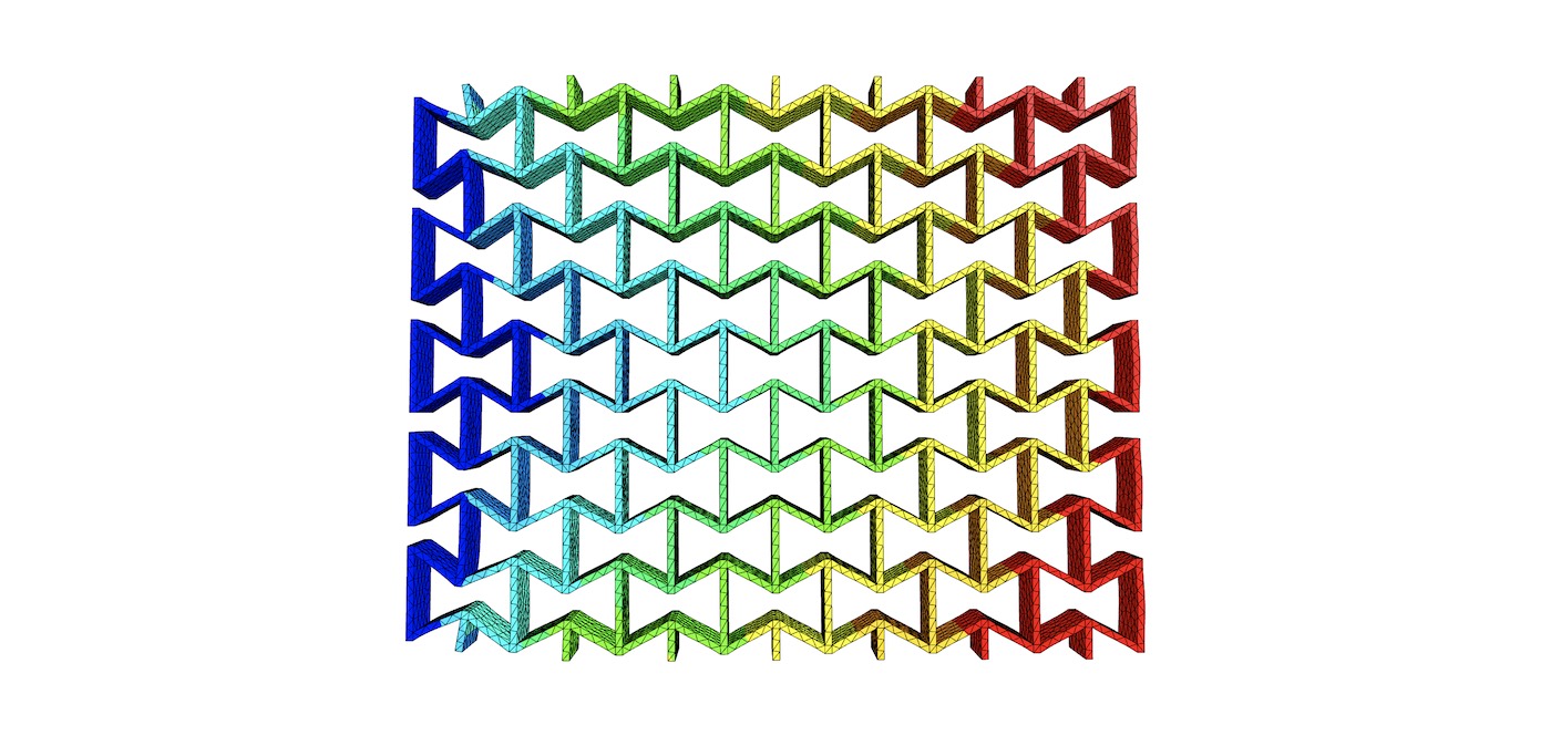
Design a re-entrant auxetic structure, simulate it with FEM, and 3D print it in TPU.

This project (with exceptions) is published under the CC Attribution-ShareAlike 4.0 International License.