Sample higher-dimensional noise on a closed path to generate seamlessly looping procedural animations.
blog.hirnschall.net


This week we'll simulate the flow of particles through a vectorfield. As always we'll use p5js as it makes drawing and animating easy. If you are not yet comfortable with classes in javascript, you can take a look at our last Coding Challenge #2 where we took a look at the basics.
If you are interested in the mathematical background of this weeks challenge make sure to check out the Mathematical Background section below.
Ok, so we want to simulate the flow of particles through a vecotfield. But what is a Vectorfield?
A vectorfield maps each point \((x,y)\) to a vector. To simulate the flow of particles we'll do the following:
While this might sound difficult it is actually quite easy. Lets take a quick look at how to generate a vectorfield before we start with the code.
If we assign a random vector to each point \((x,y)\) the resulting "flow" will look very bad. What we want is a more like a river where the direction of flow cannot change instantaneous. We can do this by using perlin noise. If you are not familiar with perlin noise take a look at this article I wrote. In short, perlin noise is a more controlled form of randomness.
So, the plan is to use 2d perlin nosie to generate a random number between \(0\) and \(1\) based on the position \((x,y)\) of the particle and then map the result to a value from \(0\) to \(360\). We can interpret this value as the direction of the vector (angle). Now that that's out of the way lets take a look at the implementation:
As we want multiple particles we'll start with particle class that..
function Particle(x, y) {
    this.x = x;
    this.y = y;
    this.v = [-1,0];

    this.show = function () {
        fill(200)
        ellipse(this.x,this.y,5,5);
    }

    this.update = function(){
        this.v=[cos(noise(this.x/s,this.y/s)*TWO_PI),sin(noise(this.x/s,this.y/s)*TWO_PI)];
        this.x += this.v[0]*particlespeed;
        this.y += this.v[1]*particlespeed;
        //check if particle has reached left end
        if(this.x<-10){
            this.x=canvasWidth+10;
            this.y=random(canvasHeight);
        }
    }
}
The show function is very simple so lets start with the update function. To map the noise value to a direction we multiply it by \(2\pi\) which is \(360\) degrees in radians. We then take the cosine to get the \(x\)-value and the sine to get the \(y\)-value of a vector with length one that is pointing in the desired direction. We can then add this "velocity" vector to the current position.
If the particle reaches the left end of the canvas we will reset its position.
function draw(){
    if(particlesc < maxparticles && frameCount%10==0)
particles[particlesc++] = new Particle(canvasWidth+10,random(canvasHeight)); for(var i=0;i<particlesc;++i){
particles[i].update();
particles[i].show();
}
}That's it! This was a very short coding challenge but I think we got more comfortable with object oriented programming. As always you can download the code below and use the further ideas section to get some inspiration on how to upgrade the code on your own.
But first, lets take a look at the mathematical background of this challenge as we might use it in other projects:
As we have already mentioned above the "flowfield" we are generating is a continuous vector field \(F(x,y)\). By simulating the flow of particles through this field we are numerically calculating so called integral curves. You can see the integral curves the particles follow in the figure below:
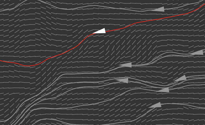
Each integral curve \(\gamma_p\) is a solution to the initial value problem
$$\gamma_p(t_0)=p$$
$$\gamma_p'(t)=F(\gamma(t)), \forall t\in I$$
Where \(p\) is the initial position of the particle. By the theorem of Peano we know that a solution \(\gamma_p\) exists for each \(p\).
If you are interested in more details feel free to ask or take a look at the wikipedia article on vector fields.
You could try to:
Sample higher-dimensional noise on a closed path to generate seamlessly looping procedural animations.

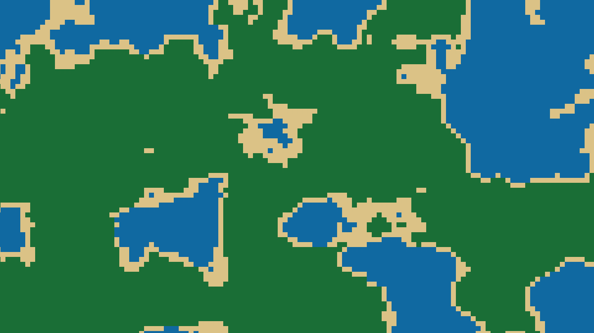
How Perlin noise generates smooth randomness — gradient vs value noise, cost, and use in terrain generation and animation.

This project (with exceptions) is published under the CC Attribution-ShareAlike 4.0 International License.

