Sample higher-dimensional noise on a closed path to generate seamlessly looping procedural animations.
blog.hirnschall.net


Perlin noise is a type of gradient noise that can be used to generate "smooth" randomness in one or more dimensions. This is why it is often used in the movie and special effects industry for procedural texture generation. It was developed by Ken Perlin in 1983. He was later awarded an Academy Award for Technical Achievement for creating the algorithm.


As you can see in fig 1.1 \(noise(x),x\in\mathbb{R}\) is a continuous function. In other words, Perlin noise can be used to generate a more "controlled" form of randomness.
To generate the random, continuous function \(noise(x):\mathbb{R}^n\to\mathbb{R}^n\) we start with a set of random vectors (gradients)
$$g_u\in\mathbb{R}^n,u\in\mathbb{Z}^n.$$As the name gradient noise implies we now set
$$noise'(u)=g_u$$ $$noise(u)=0.$$We can now interpolate to find \(noise(x),\forall x\in\mathbb{R}^n\).

As you can see in fig. 2.1 the resulting function \(noise(x)\) is zero if \(x=u\). To get a better result we take a linear combination of \(M\) weighted noise functions with different frequencies
$$Noise(x)=\sum_{i=0}^{M-1}a_i\cdot noise(f_i\cdot x)$$where \(a_i\) is a weight (amplitude) and \(f_i\) is a frequency. These terms are called octaves.


The apparently "often confused with" value noise works in a similar way to gradient noise. We start with a grid of random points
$$g_u\in\mathbb{R}^n,u\in\mathbb{Z}^n.$$In contrast to gradient noise we demand that
$$noise(u)=g_u.$$ As with gradient noise, we then use the interpolant to calculate \(noise(x),x\in\mathbb{R}^n\). To get a better result we can use a linear combination of \(M\) different octaves (with different weights, \(a_i\) and frequencies \(f_i\)). $$Noise(x)=\sum_{i=0}^{M-1}a_i\cdot noise(f_i\cdot x)$$In short: As gradient (Perlin) noise emphasizes frequencies around and above the grid spacing it will, in general, lead to a visually more appealing result.
One problem with value noise can be its random nature. The result might look ugly if too many gridpoints have a similar value.
For more information on gradient noise vs value noise take a look at this answer on StackExchange.
As we have seen above, to evaluate \(noise(x),x\in\mathbb{R}^n\) (n-dimensional Perlin noise), we have to interpolate between the \(2^n\) nearest grid points. We will later see that this can be done by calculating the dot-product of the gradient assigned to each of these points and \(x\). Afterward, we interpolate linearly between the results and apply an ease curve.
As all of these operations scale with complexity \(\mathcal{O}(n)\) the algorithm scales with complexity \(\mathcal{O}(2^n)\) for \(n\) dimensions.
Perlin noise is typically used to make things look more realistic or live like. As most things in nature do not change instantaneous, using a normal random number generator is not a good option. As we have seen Perlin noise is a continuous ("smooth") function and therefore the result looks much more natural.
For more flexibility, we may use different dimensions of Perlin noise. You can see some example use cases below:
| Dimension | Visualization | Example usage |
|---|---|---|
| 1 |
|
1d Perlin noise can be used to make a straight line look hand-drawn or make movement look more realistic (no instant speed changes, no perfectly straight lines, etc.) |
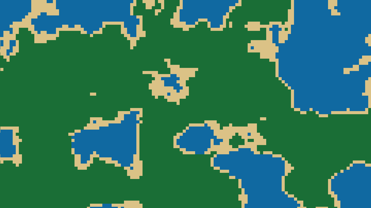
| 2 |

|

2d Perlin noise is often used to generate terrain, textures, or flowfields. |
| 3 |

|

3d Perlin noise can be used to generate caves (like those in Minecraft) or for animating textures etc. that use 2d noise |
If the language you are using does not have Perlin noise as a built-in function you can either use Ken Perlin's reference implementation to implement it yourself or check github.com if someone else already did all the work.
If you are using unity you can use Mathf.PerlinNoise(float x, float y).
In contrast to \(random()\), \(noise(t)\) will return the same value for a given \(t\) no matter how often we call it. To get different results we increment \(t\). We can control the smoothness by how quickly we increment \(t\).

If we need more than one noise value \(x:=noise(t_1)\) and \(y:=noise(t_2)\) we can use a large offset between \(t_1\) and \(t_2\). You can see how this works in fig. 3.2 below:

Depending on the implementation the noise function will return a value \(x\) in a given intervall\([a,b],a<b\). This is not what we want for most usecases. If we want a value between \(c\) and \(d\) with \(c<d\), we can map the intervall \([a,b]\) to \([c,d]\) using
$$map(x,a,b,c,d) := \frac{(x-a)(d-c)}{b-a}+c.$$Some languages have this function already implemented (p5js for example).
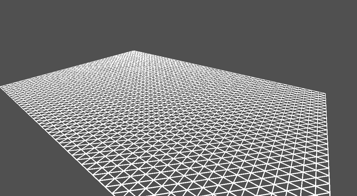
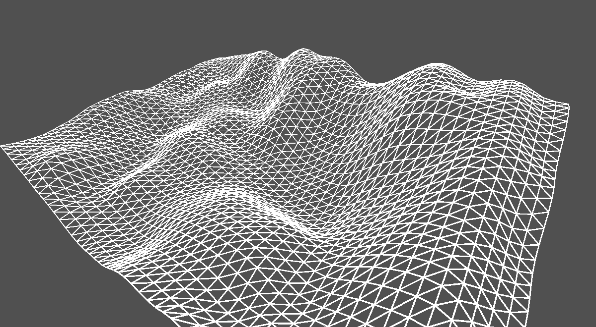
Let's start with a triangulation of a plane (fig. 3.3 (a)). We can now use 2d Perlin noise to assign a random z value (height) to each vertex (x,y). To control the smoothness we can divide both x and y by some constant s. We will also map the result of noise(x,y), a value between 0 and 1 (in p5js), to a value between minheight and maxheight to control the min and max height of the terrain we generate. You can see the result in fig. 3.3 (b).
    for(var y =0;y<height/w;++y){
  beginShape(TRIANGLE_STRIP);
  for(var x =0;x<=width/w;++x){
    vertex(x*w,j*w,map(noise(x/s,y/s),0,1,minheight,maxheight));
    vertex(x*10,(y+1)*w,map(noise(x/s,(y+1)/s),0,1,minheight,maxheight));
  }
  endShape();
}
Using the example above we'll start with a terrain (or texture) \(T=(x,y,noise(x,y)):x\in[a,b],y\in[c,d]\). If you are not familiar with this notation, it means the terrain (or texture) \(T\) is a set of points \((x,y)\) and their corresponding noise value \(noise(x,y)\). If we want this terrain (or texture) to change smoothly we can:
Sample higher-dimensional noise on a closed path to generate seamlessly looping procedural animations.
Convert Gerber files to a simulation-ready STEP file with full copper geometry (defeatured) — free tool for EM simulation.

This project (with exceptions) is published under the CC Attribution-ShareAlike 4.0 International License.